Insertion sort

sorted part and unsorted part
pseudocode
FOR Pointer ← 1 TO NumberOfitems – 1
    ItemToBeInserted ← List[Pointer]
    CurrentItem ← Pointer – 1 // pointer to last item in sorted part of list
    WHILE (List[CurrentItem] > ItemToBeInserted) AND (CurrentItem > –1) DO
        List[CurrentItem + 1] ← List[CurrentItem] // move current item down
        CurrentItem ← CurrentItem – 1 // look at the item above
    ENDWHILE
    List[CurrentItem + 1] ← ItemToBeInserted // insert item
NEXT Pointer
Binary Search
Binary search: repeated checking of the middle item in an ordered search list and discarding the half of the list which does not contain the search item
Pseudocode
Found ← FALSE
SearchFailed ← FALSE
First ← 0
Last ← MaxItems – 1 // set boundaries of search area
WHILE NOT Found AND NOT SearchFailed DO
    Middle ← (First + Last) DIV 2 // find middle of current search area
    IF List[Middle] = SearchItem
        THEN
            Found ← TRUE
        ELSE
            IF First >= Last // no search area left
                THEN
                    SearchFailed ← TRUE
                ELSE
                    IF List[Middle] > SearchItem
                        THEN // must be in first half
                            Last ← Middle - 1 // move upper boundary
                        ELSE // must be in second half
                            First ← Middle + 1 // move lower boundary
                    ENDIF
            ENDIF
    ENDIF
ENDWHILE
IF Found = TRUE
    THEN
        OUTPUT Middle // output position where item was found
    ELSE
        OUTPUT "Item not present in array"
ENDIF
Linked List

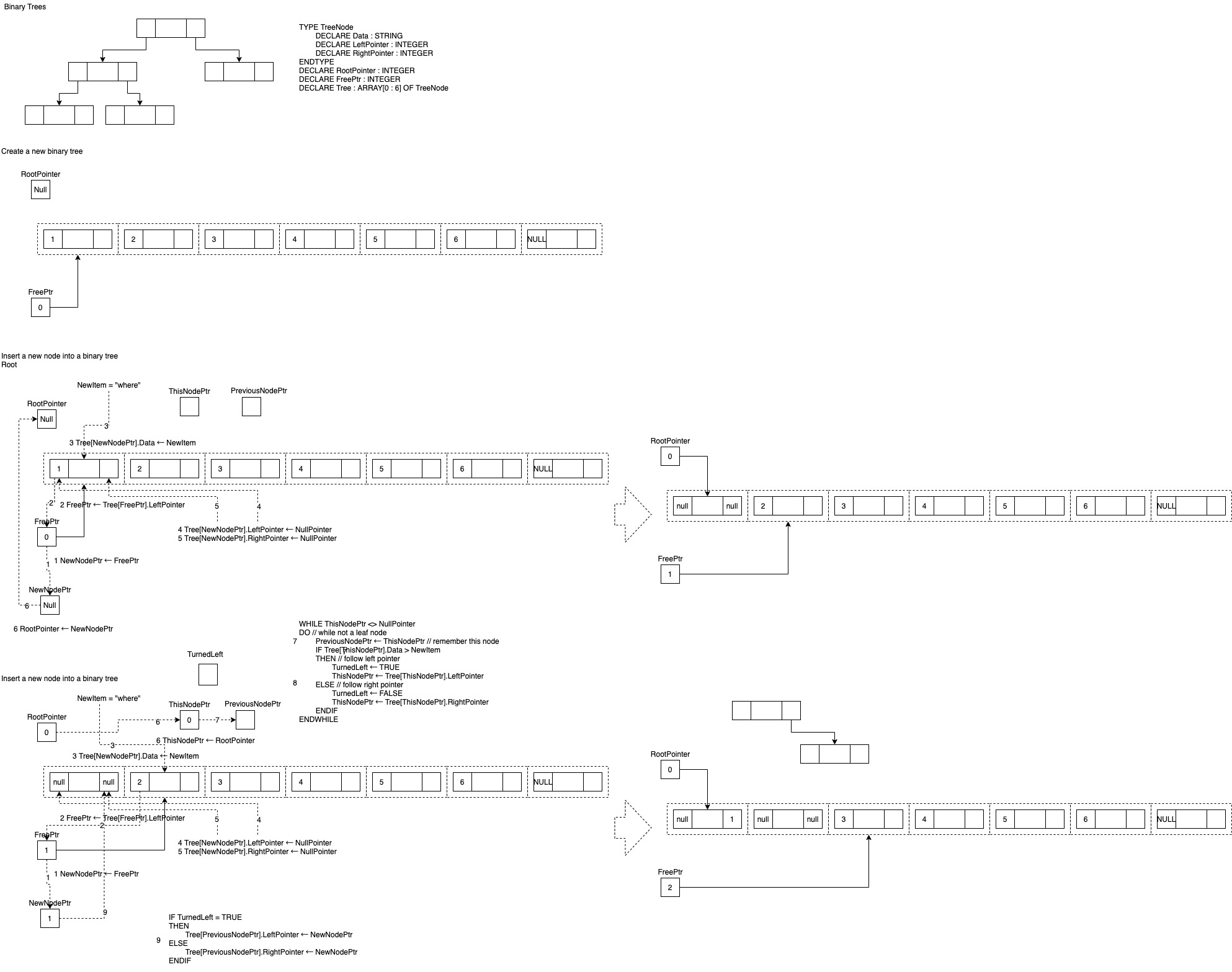
Binary Trees
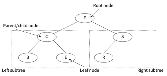
Nodes are added to an ordered binary tree\ (Structure English):
Start at the root node as the current node.
Repeat
    If the data value is greater than the current node’s data value, follow the right branch.
    If the data value is smaller than the current node’s data value, follow the left branch.
Until the current node has no branch to follow.
Add the new node in this position.
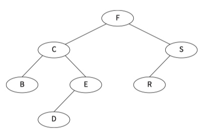
Example :: add a new node with data value D to the binary tree
- Start at the root node.
- D is smaller than F, so turn left.
- D is greater than C, so turn right.
- D is smaller than E, so turn left.
- There is no branch going left from E, so we add D as a left child from E
Store the binary tree in an array of records.
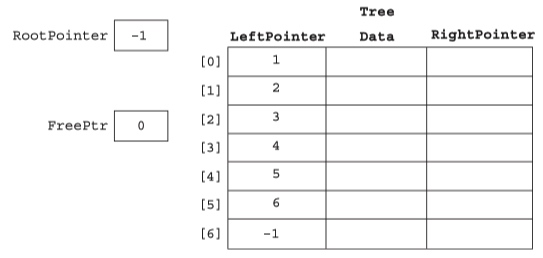
binary tree algorithm
Stacks
A stack can be implemented using a 1D array.

Queues
A queue can be implemented using a 1D array.

Graphs
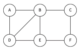
Graphic
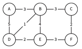
Weighted graphic
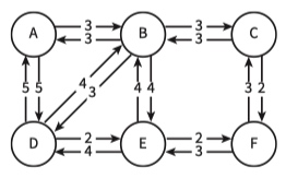
Directed graph
In Computer Science a graph is an ADT consisting of vertices (nodes) and edges.
A labelled(Weighted) graph has edges with values representing something.
Graphs can be directed or undirected.
To implement a graph, we can use an adjacency matrix or an adjacency list
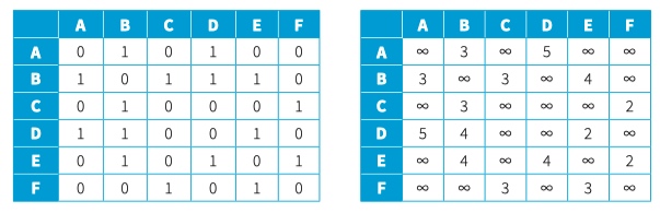
For an unweighted graph, a 1 represents an edge, a 0 no edge. When weights are to be recorded, the weight replaces the 1. Instead of a 0, we use the infinity symbol ∞.
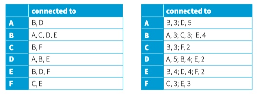
An adjacency list stores the relationship between every vertex to all relevant vertices. An entry is made only when there is an edge between two vertices.
23.13 Big O notation

A problem can be solved in different ways, with different algorithms.
Clearly, we want to use time and memory efficiently. A way of comparing the efficiency of algorithms has been devised using order of growth as a function of the size of the input.
Big O notation is used to classify algorithms according to how their running time (or space requirements) grows as the input size grows. The letter O is used because the growth rate of a function is also referred to as ‘order of the function’. The worst-case scenario is used when calculating the order of growth for very large data sets.